Kernel Density Estimation and (re)sampling
![]()
![]()

![]()
![]()
This package performs KDE operations on multidimensional data to: 1) calculate estimated PDFs (probability distribution functions), and 2) resample new data from those PDFs.
A number of examples (also used for continuous integration testing) are included in the package notebooks. Some background information and references are included in the JOSS paper.
Full documentation is available on kalepy.readthedocs.io.
pip install kalepy
git clone https://github.com/lzkelley/kalepy.gitpip install -e kalepy/
In this case the package can easily be updated by changing into the source directory, pulling, and rebuilding:
cd kalepygit pullpip install -e .# Optional: run unit tests (using the `pytest` package)pytest
import numpy as npimport matplotlib.pyplot as pltimport matplotlib as mplimport kalepy as kalefrom kalepy.plot import nbshow
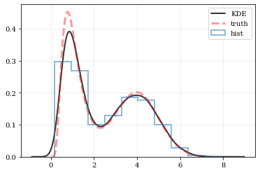
Generate some random data, and its corresponding distribution function
NUM = int(1e4)np.random.seed(12345)# Combine data from two different PDFs_d1 = np.random.normal(4.0, 1.0, NUM)_d2 = np.random.lognormal(0, 0.5, size=NUM)data = np.concatenate([_d1, _d2])# Calculate the "true" distributionxx = np.linspace(0.0, 7.0, 100)[1:]yy = 0.5*np.exp(-(xx - 4.0)**2/2) / np.sqrt(2*np.pi)yy += 0.5 * np.exp(-np.log(xx)**2/(2*0.5**2)) / (0.5*xx*np.sqrt(2*np.pi))
# Reconstruct the probability-density based on the given data points.points, density = kale.density(data, probability=True)# Plot the PDFplt.plot(points, density, 'k-', lw=2.0, alpha=0.8, label='KDE')# Plot the "true" PDFplt.plot(xx, yy, 'r--', alpha=0.4, lw=3.0, label='truth')# Plot the standard, histogram density estimateplt.hist(data, density=True, histtype='step', lw=2.0, alpha=0.5, label='hist')plt.legend()nbshow()
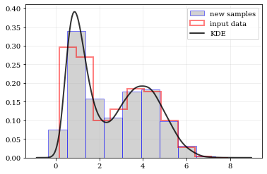
Draw a new sample of data-points from the KDE PDF
# Draw new samples from the KDE reconstructed PDFsamples = kale.resample(data)# Plot new samplesplt.hist(samples, density=True, label='new samples', alpha=0.5, color='0.65', edgecolor='b')# Plot the old samplesplt.hist(data, density=True, histtype='step', lw=2.0, alpha=0.5, color='r', label='input data')# Plot the KDE reconstructed PDFplt.plot(points, density, 'k-', lw=2.0, alpha=0.8, label='KDE')plt.legend()nbshow()
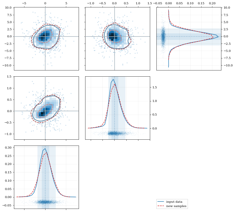
reload(kale.plot)# Load some random-ish three-dimensional datanp.random.seed(9485)data = kale.utils._random_data_3d_02(num=3e3)# Construct a KDEkde = kale.KDE(data)# Construct new data by resampling from the KDEresamp = kde.resample(size=1e3)# Plot the data and distributions using the builtin `kalepy.corner` plotcorner, h1 = kale.corner(kde, quantiles=[0.5, 0.9])h2 = corner.clean(resamp, quantiles=[0.5, 0.9], dist2d=dict(median=False), ls='--')corner.legend([h1, h2], ['input data', 'new samples'])nbshow()
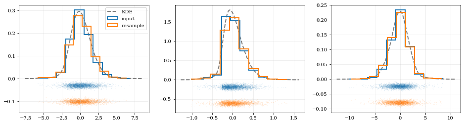
# Resample the data (default output is the same size as the input data)samples = kde.resample()# ---- Plot the input data compared to the resampled data ----fig, axes = plt.subplots(figsize=[16, 4], ncols=kde.ndim)for ii, ax in enumerate(axes):# Calculate and plot PDF for `ii`th parameter (i.e. data dimension `ii`)xx, yy = kde.density(params=ii, probability=True)ax.plot(xx, yy, 'k--', label='KDE', lw=2.0, alpha=0.5)# Draw histograms of original and newly resampled datasets*_, h1 = ax.hist(data[ii], histtype='step', density=True, lw=2.0, label='input')*_, h2 = ax.hist(samples[ii], histtype='step', density=True, lw=2.0, label='resample')# Add 'kalepy.carpet' plots showing the data points themselveskale.carpet(data[ii], ax=ax, color=h1[0].get_facecolor())kale.carpet(samples[ii], ax=ax, color=h2[0].get_facecolor(), shift=ax.get_ylim()[0])axes[0].legend()nbshow()
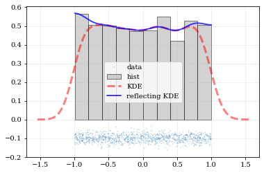
What if the distributions you’re trying to capture have edges in them, like in a uniform distribution between two bounds? Here, the KDE chooses ‘reflection’ locations based on the extrema of the given data.
# Uniform data (edges at -1 and +1)NDATA = 1e3np.random.seed(54321)data = np.random.uniform(-1.0, 1.0, int(NDATA))# Create a 'carpet' plot of the datakale.carpet(data, label='data')# Histogram the dataplt.hist(data, density=True, alpha=0.5, label='hist', color='0.65', edgecolor='k')# ---- Standard KDE will undershoot just-inside the edges and overshoot outside edgespoints, pdf_basic = kale.density(data, probability=True)plt.plot(points, pdf_basic, 'r--', lw=3.0, alpha=0.5, label='KDE')# ---- Reflecting KDE keeps probability within the given bounds# setting `reflect=True` lets the KDE guess the edge locations based on the data extremapoints, pdf_reflect = kale.density(data, reflect=True, probability=True)plt.plot(points, pdf_reflect, 'b-', lw=2.0, alpha=0.75, label='reflecting KDE')plt.legend()nbshow()
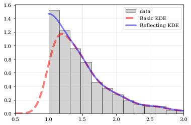
Explicit reflection locations can also be provided (in any number of dimensions).
# Construct random data, add an artificial 'edge'np.random.seed(5142)edge = 1.0data = np.random.lognormal(sigma=0.5, size=int(3e3))data = data[data >= edge]# Histogram the data, use fixed bin-positionsedges = np.linspace(edge, 4, 20)plt.hist(data, bins=edges, density=True, alpha=0.5, label='data', color='0.65', edgecolor='k')# Standard KDE with over & under estimatespoints, pdf_basic = kale.density(data, probability=True)plt.plot(points, pdf_basic, 'r--', lw=4.0, alpha=0.5, label='Basic KDE')# Reflecting KDE setting the lower-boundary to the known value# There is no upper-boundary when `None` is given.points, pdf_basic = kale.density(data, reflect=[edge, None], probability=True)plt.plot(points, pdf_basic, 'b-', lw=3.0, alpha=0.5, label='Reflecting KDE')plt.gca().set_xlim(edge - 0.5, 3)plt.legend()nbshow()
# Load a predefined dataset that has boundaries at:# x: 0.0 on the low-end# y: 1.0 on the high-enddata = kale.utils._random_data_2d_03()# Construct a KDE with the given reflection boundaries given explicitlykde = kale.KDE(data, reflect=[[0, None], [None, 1]])# Plot using default settingskale.corner(kde)nbshow()
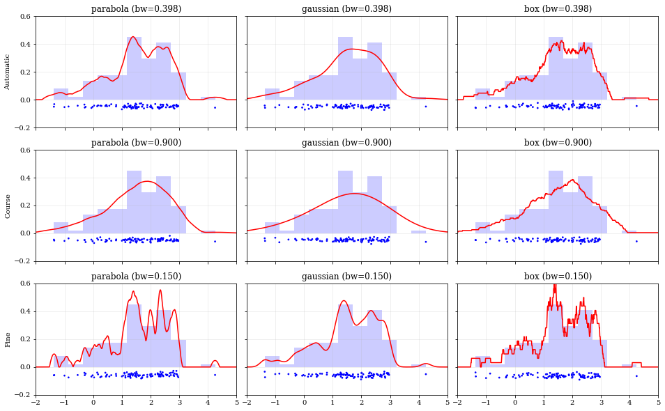
# Load predefined 'random' datadata = kale.utils._random_data_1d_02(num=100)# Choose a uniform x-spacing for drawing PDFsxx = np.linspace(-2, 8, 1000)# ------ Choose the kernel-functions and bandwidths to test ------- #kernels = ['parabola', 'gaussian', 'box'] #bandwidths = [None, 0.9, 0.15] # `None` means let kalepy choose ## ----------------------------------------------------------------- #ylabels = ['Automatic', 'Course', 'Fine']fig, axes = plt.subplots(figsize=[16, 10], ncols=len(kernels), nrows=len(bandwidths), sharex=True, sharey=True)plt.subplots_adjust(hspace=0.2, wspace=0.05)for (ii, jj), ax in np.ndenumerate(axes):# ---- Construct KDE using particular kernel-function and bandwidth ---- #kern = kernels[jj] #bw = bandwidths[ii] #kde = kale.KDE(data, kernel=kern, bandwidth=bw) ## ---------------------------------------------------------------------- ## If bandwidth was set to `None`, then the KDE will choose the 'optimal' valueif bw is None:bw = kde.bandwidth[0, 0]ax.set_title('{} (bw={:.3f})'.format(kern, bw))if jj == 0:ax.set_ylabel(ylabels[ii])# plot the KDEax.plot(*kde.pdf(points=xx), color='r')# plot histogram of the data (same for all panels)ax.hist(data, bins='auto', color='b', alpha=0.2, density=True)# plot carpet of the data (same for all panels)kale.carpet(data, ax=ax, color='b')ax.set(xlim=[-2, 5], ylim=[-0.2, 0.6])nbshow()
weights
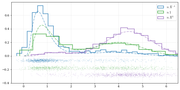
# Load some random data (and the 'true' PDF, for comparison)data, truth = kale.utils._random_data_1d_01()# ---- Resample the same data, using different weightings ---- #resamp_uni = kale.resample(data, size=1000) #resamp_sqr = kale.resample(data, weights=data**2, size=1000) #resamp_inv = kale.resample(data, weights=data**-1, size=1000) ## ------------------------------------------------------------ ## ---- Plot different distributions ----# Setup plotting parameterskw = dict(density=True, histtype='step', lw=2.0, alpha=0.75, bins='auto')xx, yy = truthsamples = [resamp_inv, resamp_uni, resamp_sqr]yvals = [yy/xx, yy, yy*xx**2/10]labels = [r'$\propto X^{-1}$', r'$\propto 1$', r'$\propto X^2$']plt.figure(figsize=[10, 5])for ii, (res, yy, lab) in enumerate(zip(samples, yvals, labels)):hh, = plt.plot(xx, yy, ls='--', alpha=0.5, lw=2.0)col = hh.get_color()kale.carpet(res, color=col, shift=-0.1*ii)plt.hist(res, color=col, label=lab, **kw)plt.gca().set(xlim=[-0.5, 6.5])# Add legendplt.legend()# display the figure if this is a notebooknbshow()
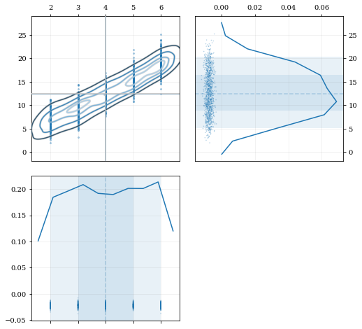
# Construct covariant 2D dataset where the 0th parameter takes on discrete valuesxx = np.random.randint(2, 7, 1000)yy = np.random.normal(4, 2, xx.size) + xx**(3/2)data = [xx, yy]# 2D plotting settings: disable the 2D histogram & disable masking of dense scatter-pointsdist2d = dict(hist=False, mask_dense=False)# Draw a corner plotkale.corner(data, dist2d=dist2d)nbshow()
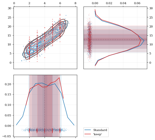
A standard KDE resampling will smooth out the discrete variables, creating a smooth(er) distribution. Using the keep parameter, we can choose to resample from the actual data values of that parameter instead of resampling with ‘smoothing’ based on the KDE.
kde = kale.KDE(data)# ---- Resample the data both normally, and 'keep'ing the 0th parameter values ---- #resamp_stnd = kde.resample() #resamp_keep = kde.resample(keep=0) ## --------------------------------------------------------------------------------- #corner = kale.Corner(2)dist2d['median'] = False # disable median 'cross-hairs'h1 = corner.plot(resamp_stnd, dist2d=dist2d)h2 = corner.plot(resamp_keep, dist2d=dist2d)corner.legend([h1, h2], ['Standard', "'keep'"])nbshow()
Please visit the github page <https://github.com/lzkelley/kalepy>_ for issues or bug reports. Contributions and feedback are very welcome.
Contributors:
JOSS Paper:
A JOSS paper has been submitted. If you have found this package useful in your research, please add a reference to the code paper:
.. code-block:: tex
@article{kalepy,author = {Luke Zoltan Kelley},title = {kalepy: a python package for kernel density estimation and sampling},journal = {The Journal of Open Source Software},publisher = {The Open Journal},}