Study-09-MachineLearning-D

DeepLearning (CNN, RNN)

CNN

Applications ?

• ComputerVision
• NaturalLanguageProcessing (WaveNet-model)
• Let SelfDrivingCars read Road Signs
• limitless….

Introduction with MNIST database

As arguably the most famous database in the field of deep learning, it contains 70,000 images of hand-written digits(0-9).

from keras.datasets import mnist
(X_train, y_train), (X_test, y_test) = mnist.load_data()

Sometimes some digits are less legible than others. How to conquer these difficulty? How our algorithm examine the images and discover patterns? These pattern can then be used to decipher the digits in images that it hasn’t seen before. Let’s see how computer sees when we input these images.

1. [MLP]

X

For computer, an image is a matrix with one entry for each image pixel. Each image in MNIST database is 28 x 28(pixel). White pixels are encoded as 255, black pixels are encoded as 0, and grey pixels appear in the matrix as an integer somewhere in between. We rescale each image to have values in the range from 0 to 1.

y

Before supplying the data to our deeplearning network, we’ll need to preprocess the labels(y_train, y_test) because each image currently has a label that’s integer-valued. So we convert this to an one-hot encoding. Each label will be transformed to a vector with mostly 0.

X again?

However, recall that our MLP only takes vectors as input. So if we want to use MLP with images, we have to first convert all of our matirces to vectors. For example, in the case of a 28 x 28 image, we can get a vector with 784 entries. This is called flattening. After encoding our images as vectors, they can be fed into the input layer of our MLP.

How to create our MLP for discovering the patterns in our data? Let’s say…

• Since our data pt are vectors with 784 entries -> the input layer with 784 nodes
• Let’s say -> the 2 hidden layers each containing 572 nodes
• The model needs to distinguish 10 different digits -> the output layer with 10 nodes, activation=’softmax’
  • the softmax function ensures that our network outputs an estimate for the probability that each potential digit is depicted in the image(multi-class classification).

Here, we just add the ‘flatten layer’ before we specify our MLP. It takes the image matrix’s input and convert it to a vector.

After first fitting…

This model is great as a first draft, but we can make it better.

• To lift model accuracy:
  • add ‘relu’ activation function to all of our hidden layers. ‘relu’ helps with the vanishing gradients problem.
• To minimize overfitting:
  • add dropout layer. This layer must be supplied a parameter(from 0 to 1) which is a probability that any node in the network is dropped during training.
    

Now our data is processed and our model is specified. Currently, all of the 600,000 weights have random values so the model has random predictions. By training our model, we’ll modify these weights and improve predictions. Before training the model, we need to specify a loss function. Since we are constructing a multi-class classifier, we will use categorical_crossentropy loss function.

categorical_crossentropy

This loss function checks to see if our model has done a good job with classifying an image by comparing the model’s predictions to the true label. As seen above, each label became a vector with 10 entries. Our model outputs a vector also with 10 entries which are predictions.

• Here our model predicts there’s an ‘8’ in the image with 90% probability and a ‘3’ in the image with 10% probability. But in the label, there is a 100% probability that the imagedepicts a ‘3’.
• the categorical_crossentropy_loss looks at these two vectors and returns a lower value if the two vectors agree regarding what’s in the image.
  

In this example, our model is pretty sure that the digit is an ‘8’, but the label knows for certain it’s a ‘3’ thus, will return a higher value for the loss. If the model later returns the next output where it changes to being 90% sure thata the image depicts a ‘3’ the loss value will be lower. To sum, if the model predictions agree with the labels, the loss is lower.

We want its predictions to agree with the labels. We’ll try to find the model parameters that gives us predictions that minimizing the loss function. And the standard method for descending a loss function is called Gradient Descent. There are lots of ways to perform Gradient Descent and each method in Keras has a corresponding optimizer. The surface depicted here is an example of a loss function and all of the optimizers are racing towards the minimum of the function, and some are better than others.

Compiling_Step

• we’ll specify the ‘loss’, ‘optimizer’, and ‘metrics’.

  For loss function…

  • ‘mean_squared_error’ (y_true, y_pred)
  • ‘binary_crossentropy’ (y_true, y_pred)
  • ‘categorical_crossentropy’ (y_true, y_pred), etc…

For optimizer…

• ‘sgd’ : Stochastic Gradient Descent
• ‘rmsprop’ : RMSprop (for recurrent neural networks??)
• ‘adagrad’ : Adagrad that adapts learning rates, accumulating all past gradients?
• ‘adadelta’ : a more robust extension of Adagrad that adapts learning rates based on a moving window of gradient updates?
• ‘adam’ : Adam
• ‘adamax’ : Adamax
• ‘nadam’ : Nesterov Adam optimizer
• ‘tfoptimizer’ : TFOptimizer

Training_Step

To understand the modification of training code, we’ll first need to understand the idea of ‘model validation’. So far, we’ve checked model performance based on how the loss in accuracy changed with epoch. When we design our model, it’s not always clear how many layers the network should have or how many nodes to place in each layer or how many epochs and what batch_size should we use. So we break our dataset into three set: train + validation + test. Our model looks only at the training set when deciding how to modify its weights. And every epoch, the model checks how it’s doing by checking its accuracy on the validation set (but it does not use any part of the validation set for the backpropagation step). We use the training set to find all the patterns we can, and the validation set tells us if our chosen model is performing well. Since our model does not use the validation set for deciding the weights, it can tell us if we’re overfitting to the training set. For example, around certain epoch, we can get some evidence of overfitting where the **training loss** starts to decrease but the **validation loss** starts to increase. Then we will want to keep the weights around the epoch and discard the weights from the later epochs. This kind of process can prove useful if we have multiple potential architectures to choose from.

• How many layers? nodes? epochs? batch_size?: we save the weights from each potential architecture for later comparison. Then we will always pick the model that gets the lowest validation loss.
• but why we create the test set?: When we go to test the model, it looks at data that it has truly never seen before. Eventhough the model doesn’t use the validation set to update its weights, our model selection process can be biased in favor of the validation set.
• Notice the fit() takes validation_split argument. ModelCheckpoint() class allows us to save the model weights after each epoch. save_best_only parameter says that save the weights to get the best accuracy on the validation set.

  But in the case of real-world messy image data(random size, complex shapes, patterns..), do you think MLP works? Nope!

  • MLP only use fully connected layers…it uses too many parameters..a risk of overfitting
  • MLP only accepts vectors as input
    

2. [CNN]

[A] What’s the convolutional layer?

• Break the image up into smaller pieces.
  • first select a width and height defining a convolutional window.
  • then simply slide this window horizontally, vertically over the matrix of the pixels
  • At each position, the window specifies a small piece within the image, and define a collection of pixels to which we connect a single hidden node.

Q. In detail, how a regional collection of input nodes influences the value of a node in a convolutional layer?

• Let’s represent the weights connecting the nodes by writing a numerical value on top of the arrows.
• Then in order to get the value of a node in the convolutional layer for this image input we operate as we did with MLP with multiplying the input nodes by their corresponding weights and summing up the result. When we do that, we get zero just as with MLP (and there is a bias term, but we assume it’s ‘0’ and ignore it). We’ll always add a Relu activation function to our convolutional layers, thus in this case, our zero stays zero. Now plug in the value for our first node in the convolutional layer. The values of all other nodes in the convolutional layer are caluculated in the same way.
• Now instead of representing weights on the top of the arrows, we decided to represent them in a grid, which we will call filter. It’s size is always match the size of the convolutional window.
• Now the process of calculating the value of the nodes in the convolutional layer. In the second case, notice that the positive values in the filter perfectly correspond to the largest values in this region of the image. The converse is also true, the negative values in the filter corresponding to the smallest values in the image. In fact, since we rescaled the pixels in the image to lie b/w 0 and 1, ‘3’ is the largest we can get for this filter. That is, the pattern in this region with a diagonal white stripe down the middle, is the only arrangement of pixels that will yield this maximal value ‘3’. We can see ‘3’ also appears again, and it verifies the corresponding region in the image is identical.
• In fact, when using CNN, we should visualize our filters which will tell us what kind of pattern our filters want to detect. Just like MLP, these weights will not be set in advance and will be learned by the network as the weights that minimize our loss function. Of course, if we want to detect more patterns, we need to use more filters.
  

Q. How to perform a convolution on a color images?

• We still move a filter horizontally, vertically across the image. Only now the filter is itself 3-dimensional to have a value for each color channel at each horizontal and vertical lacation in the image array. Just like we think of the color image as a stack of three 2d matices, the same is true of our filter.

• Now to obtain the values of the nodes in the feature map corresponding to this filter, we do the same thing, but only now, our sum has over 3 times as many terms.
  

• If we want to picture the case of a color image with multiple filters, we would define multiple 3d arrays (each as a stack of 2d arrays) as our filters. Then we can think about each of the feature maps in a convolutional layer along the same lines as an image channel and stack them to get a 3d array. Then, we can use this 3d array as input to still another convolutional layer to discover patterns within the patterns that we discovered in the first convolutional layer. We can then do this again to discover patterns within patterns within patterns….
  

Both in MPL, CNN, the inference works the same way (weights, biases, loss, etc…), but

• In MLP, Dense layers are fully connected, meaning that the nodes are connected to every node in the previous layer.
• Convolutional layers
  • are locally connected where their nodes are connected to only a subset of previous layer’s nodes.
  • have this added parameter sharing.
  • the weights take the form of convolutional filters that are randomly generated, so are the patterns to detect..and while training, filters are updated at each epoch to take on values that minimize the loss function. CNN determines what kind of patterns it needs to detect based on the loss function.
  • So with CNN to emphasize, we won’t specify the values of the filters or tell the CNN what kind of patterns it needs to detect. THESE WILL BE LEARNED FROM THE DATA.

So we can control the behavior of a convolutional layer by specifying the no.of filters and the size of each filter.

• To increase the no.of nodes in a convolutional layer, we could increase the no.of filters, then we would get more feature maps(activation map).
• To increase the size of patterns, we could increase the size of each filter.

But in addition to this, there are more hyperparameters to tune.

• Stride
  • Stride refers the amount by which the filter slides (horizontally, vertically) over the image
  • One stride makes the one node in the one collection
• Padding
  • what if…we go..’stride with 2, 3, ..’and the filter(or window) extends outside the image(because the width, height are off)?
    • option_1: discarding those pixels..so no information about some regions of the image.padding='valid'
    • option_2: padding them with ‘0’..so we can get all contribution from every regions of the image. padding='same'

This is a feature extraction using a convolution with ‘3 x 3’ window and stride ‘1’.

To create a convolutional layer in Keras:

from keras.layers import Conv2D
Conv2D(filters, kernel_size, strides, padding, activation='relu', input_shape)

• filters: The number of filters.
• kernel_size: Number specifying both the height and width of the convolution window
• strides: The stride of the convolution. If you don’t specify anything, strides is set to 1
• padding: One of ‘valid’ or ‘same’. If you don’t specify anything, padding is set to ‘valid’
• activation: Typically ‘relu’. If you don’t specify anything, no activation is applied. You are strongly encouraged to add a ReLU activation function to every convolutional layer in your networks.
• input_shape: When using your convolutional layer as the first layer (appearing after the input layer) in a model, you must provide an additional input_shape argument. Tuple specifying the height, width, and depth of the original input. Do not include the input_shape argument if the convolutional layer is not the first layer in your network.

EX1> My input layer accepts grayscale images that are 200 by 200 pixels (corresponding to a 3D array with height 200, width 200, and depth 1). Then, say I’d like the next layer to be a convolutional layer with 16 filters, each with a width and height of 2. When performing the convolution, I’d like the filter to jump two pixels at a time. I also don’t want the filter to extend outside of the image boundaries; in other words, I don’t want to pad the image with zeros. Then, to construct this convolutional layer….

Conv2D(filters=16, kernel_size=2, strides=2, activation='relu', input_shape=(200, 200, 1))

EX2> I’d like the next layer in my CNN to be a convolutional layer that takes the layer constructed in Example 1 as input. Say I’d like my new layer to have 32 filters, each with a height and width of 3. When performing the convolution, I’d like the filter to jump 1 pixel at a time. I want the convolutional layer to see all regions of the previous layer, and so I don’t mind if the filter hangs over the edge of the previous layer when it’s performing the convolution. Then, to construct this convolutional layer….

Conv2D(filters=32, kernel_size=3, padding='same', activation='relu')

EX3> There are 64 filters, each with a size of 2x2, and the layer has a ReLU activation function. The other arguments in the layer use the default values, so the convolution uses a stride of 1, and the padding has been set to ‘valid’. It is possible to represent both kernel_size and strides as either a number or a tuple.

Conv2D(64, (2,2), activation='relu')

[B] What’s the pooling layer?

It takes our convolutional layers as input and reduces their dimensionality.

• A convolutional layer is a stack of feature_maps where we have one feature map for each filter. A complex dataset will require a large number of filters, each responsible for finding a pattern in the image, which means the dimensionality of our convolutional layers can get large, thus it requires more parameters…which can lead to overfitting. Thus, we need a method for reducing this dimensionality. This is where our pooling layer comes in.
• 2 types of pooling
  • Max_pooling_layer: It takes a stack of feature_maps as input. The value of the corresponding node in the max_pooling_layer is calculated by just taking the maximum of the nodes(pixels) contained in the window. From this process, the output is a stack with the same number of feature_maps, but each feature_map is reduced in width and height.
  • Global_AVG_pooling_layer: It takes a stack of feature_maps and computes the AVG value of the nodes for each map in the stack(so no need to use windows or strides). The final output is a stack of feature_maps where each is reduced to a single value. So this means it takes a 3d-array and turns it into a vector.
    

Create a max pooling layer in Keras

from keras.layers import MaxPooling2D
MaxPooling2D(pool_size, strides, padding)

• pool_size: Number specifying the height and width of the pooling window. It is possible to represent both pool_size and strides as either a number or a tuple.

EX1> I’d like to reduce the dimensionality of a convolutional layer by following it with a max pooling layer. Say the convolutional layer has size (100, 100, 15), and I’d like the max pooling layer to have size (50, 50, 15). I can do this by using a 2x2 window in my max pooling layer, with a stride of 2…

[C] CNN Architecture

• Collect millions of images and pick an image_size and resize all of our images to that same size.
• As known, any image is interpreted by the computer as a 3d_array(coz Color gives depth). We can say our input array will always be much taller(height) and wider(width) than it is deep(color). CNN architecture is designed with the goal of taking that array and making it deeper than it is taller and wide.
• Convolutional layers make the array deeper as it passes through the network
• Each of the convolutional layers requires to specify a number of hyperparameters.
  • kernal_size: from 2x2 to 5x5
  • No.of filters: It controls the depth of the convolutional layer since the convolutional layer has one activation function for each filter. (no.of filters = depth = no.of activation_func)
  • Often, we will have the no.of filters increase in the sequence.
• Pooling layers decrease the spatial dimensions.
  • Here, the convolutional layers expand the depth of the arrays from 3 to 16 to 32 to 64 while our max_pooling layers decrease the dimensions from 32 to 16 to 8 to 4.

This sequence of layers discovers the spatial patterns contained in the image. It gradually takes the spatial data and converts the array to a representation that encodes the various contents of the image where all spatial information is eventually lost (so it’s not relevant which pixel is next to what other pixels).

Once we get to the final representation, we can flatten the array to a vector and feed it to one or more fully connected MLP to determine what object is contained in the image. so it has a potential to classify objects more accurately.

EX2>

from keras.layers import Conv2D, MaxPooling2D, Flatten, Dense
model = Sequential()
model.add(Conv2D(filters=16, kernel_size=2, padding='same', activation='relu', input_shape=(32, 32, 3)))
model.add(MaxPooling2D(pool_size=2))
model.add(Conv2D(filters=32, kernel_size=2, padding='same', activation='relu'))
model.add(MaxPooling2D(pool_size=2))
model.add(Conv2D(filters=64, kernel_size=2, padding='same', activation='relu'))
model.add(MaxPooling2D(pool_size=2))
model.add(Flatten())
model.add(Dense(500, activation='relu'))
model.add(Dense(10, activation='softmax'))

The network begins with a sequence of three convolutional layers(to detect regional patterns), followed by max pooling layers. These first six layers are designed to take the input array of image pixels and convert it to an array where all of the spatial information has been squeezed out, and only information encoding the content of the image remains. The array is then flattened to a vector in the seventh layer of the CNN. It is followed by two dense(fully-connected) layers designed to further elucidate the content of the image. The final layer has one entry for each object class in the dataset, and has a softmax activation function, so that it returns probabilities.

Things to Remember

• Always add a ReLU activation function to the Conv2D layers in your CNN. With the exception of the final layer in the network, Dense layers should also have a ReLU activation function.
• When constructing a network for classification, the final layer in the network should be a Dense layer with a softmax activation function. The number of nodes in the final layer should equal the total number of classes in the dataset.

So now we just developed the classification model that can recognize if the given image presents ‘bird’,’cat’,’car’,…etc. But we have to deal with lots of irrelavant information in the image such as size, angle, location…etc. So we want our algorithm to learn invariant representation of of the image!

• Let it determine not based on size: scale_invariance
• Let it determine not based on angle: rotation_invariance
• Let it determine not based on the position: translation_invariance

Data Augmentation

CNN has some built-in translation invariance.

• See how we calculate Max-pooling layer. When we move the window, the value of the max pooling node would be the same as long as the maximum value stays within the window. The effect of applying many max-pooling layers in a sequence, each following a convolutional layer, is that we could translate the object quite far to the left, to the top of the image, to the bottom of the image and still our model can make sense of it all. Transforming an object?’s scale, rotation, position in the image has a huge effect on the pixel values.
• Then how our computer can conceive the differences in the image? There is a technique that makes our algorithm more statistically invariant.
  • If we want our CNN to be rotation_invariant, we add some images to our training set created by doing random rotations on our training images.
  • If we want our CNN to be translation_invariant, we add some images created by doing random translation of our training images.
    

When we do this, we see that we expand the training set by augmenting the data, and this also helps to avoid overfitting because our model is seeing many new images.

from keras.preprocessing.image import ImageDataGenerator
datagen_train = ImageDataGenerator(width_shift_range=?, height_shift_range=?, horizontal_flip=True)
datagen_train.fit(x_train)

Transfer Learning

How to adapt expert’s CNN architecture that have already learned so much about how to find the patterns in image data toward our own classification task? Do they have overlaps?

Transfer learning involves taking a pre-trained neural network and adapting the neural network to a new, different dataset. The approach for using transfer learning will be different. There are four main cases:

• new dataset is small, new data is similar to original training data
• new dataset is small, new data is different from original training data
• new dataset is large, new data is similar to original training data
• new dataset is large, new data is different from original training data

Of course, the dividing line between a large dataset and small dataset is somewhat subjective. Overfitting is a concern when using transfer learning with a small dataset.

To explain how each situation works, we will start with a generic pre-trained convolutional neural network and explain how to adjust the network for each case. Our example network contains three convolutional layers and three fully connected layers:

1> Small + Similar

• slice off the end of the neural network
• add a new fully connected layer that matches the number of classes in the new dataset
• randomize the weights of the new fully connected layer; freeze all the weights from the pre-trained network
• train the network to update the weights of the new fully connected layer
  

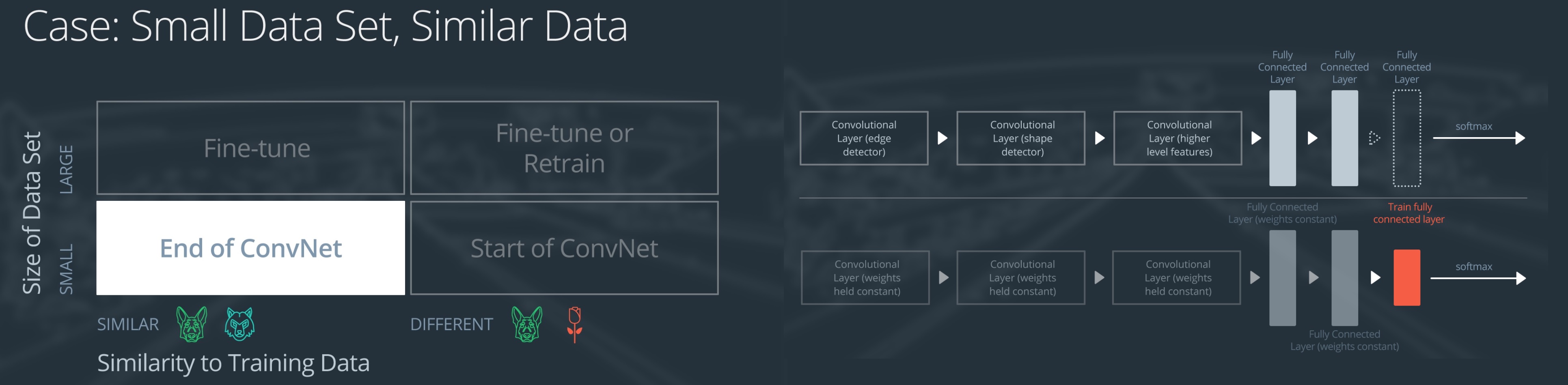
because Small:
To avoid overfitting on the small dataset, the weights of the original network will be held constant rather than re-training the weights.

because Similar:
Since the datasets are similar, images from each dataset will have similar higher level features. Therefore most or all of the pre-trained neural network layers already contain relevant information about the new dataset and should be kept.

2> Small + Different

• slice off most of the pre-trained layers near the beginning of the network
• add to the remaining pre-trained layers a new fully connected layer that matches the number of classes in the new dataset
• randomize the weights of the new fully connected layer; freeze all the weights from the pre-trained network
• train the network to update the weights of the new fully connected layer
  

because Small:
overfitting is still a concern. To combat overfitting, the weights of the original neural network will be held constant, like in the first case.

because Different:
But the original training set and the new dataset do not share higher level features. In this case, the new network will only use the layers containing lower level features.

3> Large + Similar

• remove the last fully connected layer and replace with a layer matching the number of classes in the new data set
• randomly initialize the weights in the new fully connected layer and initialize the rest of the weights using the pre-trained weights
• re-train the entire neural network
  

because Large:
Overfitting is not as much of a concern when training on a large data set; therefore, you can re-train all of the weights.

because Similar:
the original training set and the new dataset share higher level features thus, the entire neural network is used as well.

4> Large + Different

• remove the last fully connected layer and replace with a layer matching the number of classes in the new dataset
• re-train the network from scratch with randomly initialized weights
• alternatively, you could just use the same strategy as the “large and similar” data case
  

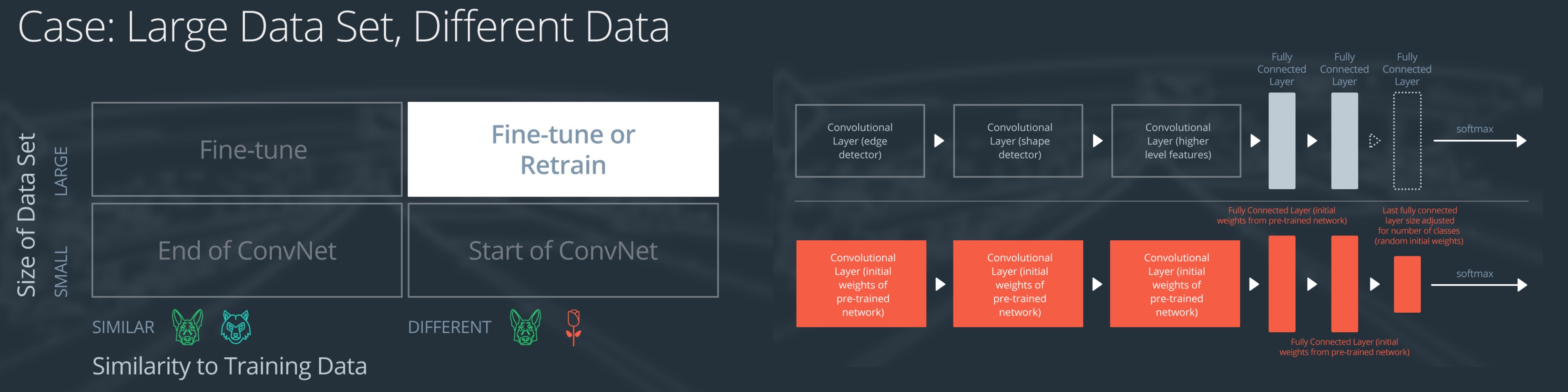
because Large and Different:
Even though the dataset is different from the training data, initializing the weights from the pre-trained network might make training faster. So this case is exactly the same as the case with a large, similar dataset.

If using the pre-trained network as a starting point does not produce a successful model, another option is to randomly initialize the convolutional neural network weights and train the network from scratch.

Example from VGG(Visual Geometry Group of Oxford)

Bayesian Neural Network

10 years ago, people used to think that Bayesian methods are mostly suited for small datasets because it’s computationally expensive. In the era of Big data, our Bayesian methods met deep learning, and people started to make some mixture models that has neural networks inside of a probabilistic model.

NN performs a given task by learning on examples without having prior knowledge about the task. This is done by finding an optimal point estimate for the weights in every node. Generally, the NN using point estimates as weights perform well with large datasets, but they fail to express uncertainty in regions with little or no data, leading to overconfident decisions.

BNNs are comprised of a Probabilistic Model and a Neural Network. The intent of such a design is to combine the strengths of Neural Networks and Stochastic modeling. NN exhibits universal continuous function approximator capabilities. Bayesian Stochastic models generate a complete posterior(constructing the distribution of the parameters) and produce probabilistic guarantees on the predictions.

• In BNNs usually, a prior is used to describe the key parameters, which are then utilized as input to a neural network. The neural networks’ output is utilized to compute the likelihood. From this, one computes the posterior of the parameters by Sampling or Variational Inference.
• But BNNs are computationally expensive, because of the sampling or variational inference steps. BNNs have been demonstrated to be competent on moderately sized datasets and not yet fully explored with vastly large datasets.

WHY BNN?

• Complexity is in the context of deep learning best understood as complex systems. Systems are ensembles of agents which interact in one way or another. These agents form together a whole. One of the fundamental characteristics of complex systems is that these agents potentially interact non-linearly. There are two disparate levels of complexity:
  • simple or restricted complexity
  • complex or general complexity
• While general complexity can, by definition, not be mathematically modelled in any way, restricted complexity can. Given that mathematical descriptions of anything more or less complex are merely models and not fundamental truths, we can directly deduce that Bayesian inference is more appropriate to use than frequentist inference. Systems can change over time, regardless of anything that happened in the past, and can develop new phenomena which have not been present to-date. This point of argumentation is again very much aligned with the definition of complexity from a social sciences angle. In Bayesian inference, we do learn the model parameters θ in form of probability distributions. Doing so, we keep them flexible and can update their shape whenever new observations of a system arrive.
• So far, there has no deterministic mathematical formalism been developed for non-linear systems and will also never be developed, because complex systems are, by definition, non-deterministic. In other words, if we repeat an experiment in a complex system, the outcome of the second experiment won’t be the same as of the first. If so.. what is the obvious path to go whenever we cannot have a deterministic solution for anything? we approximate!!! This is precisely what we do in Bayesian methods: the intractable posterior P(θ|D) is approximated, either by a variational distribution g(θ|D) in neural networks, or with Monte Carlo methods q(θ|D)(envelop) in probabilistic graphical models.
• Any deep learning model is actually a complex system by itself. We have neurons(agents), and non-linear activation functions between them(agents’ non-linear relations).

  Neural Networks are one of the few methods which can find non-linear relations between random variables.

How to BNN?
Problem: Big data?

Langevin MonteCarlo can save us?

some potential downsides in using Gibbs sampling for approximate inference in Bayesian Neural Networks

• The Gibbs sampler generates one coordinate of the weight vector w at a time, which may be very slow for neural networks with tens of millions of weights.
• The Gibbs sampler may not work with minibatching, i.e. we will have to look through the whole dataset to perform each step of the sampler. Thus, training on large datasets will be very slow.
• [note] We will have to wait until the Gibbs sampler converges and starts to produce samples from the correct distribution, but this only needs to be done on the training stage. On the test stage, we will use the weight samples collected during the training stage to predict the label for a new test object, so predicting the labels for new test samples will not be necessarily slow.

Dynamic Bayesian Neural Network