Algorithmic Portfolio Hedging. Black-Scholes Pricing for Dynamic Hedges to produce a Dynamic multi-asset Portfolio Hedging with the usage of Options contracts.
In this project it is discussed how to construct a Dynamic multi-asset Portfolio Hedging with the usage of Options contracts.
NVDA boomed over the last 2 years and here is discussed how to hedge a short position in NVDA calls.
The aim is to hedge the exposure to changes in volatility, movements in the underlying asset and the speed of movements in the underlying asset.
Options have exposure to not only the underlying asset but also interest rates, time, and volatility.
These exposures are inputs to the Black-Scholes option pricing model.
While building the script, it is also explored the intuition behind the Black-Scholes model.
Folder structure:
Dynamic-Derivatives-Portfolio-Hedging/deliverables/asset-allocation.pysrc/utils.pyvariables.pyREADME.md
In the file ../src/variables.py are set all the different variables that for a dynamic hedge needs to be updated daily.
Feel free to play with these variables and create different settings.
# main variables# asset_price : underlying price# sigma : implied volatility to insert for the BS model# dt : time to expiration# rf : risk free rate (30 day LIBOR rate)# nContract1 : number of contracts# K1 : strike price option 1# K2 : strike price option 2# K3 : strike price option 3# underlyingasset_price = 543# input BSsigma = 0.53dt = 30/365rf = .015# option 1nContract1 = -1000K1 = 545# option 2K2 = 550# option 3K3 = 570
In the file ../src/utils.py is described the model to price the European Options with the BS model.
The following code models European calls:
import mathfrom scipy.stats import norm# define the European call optionclass EuropeanCall:def call_price(self, asset_price, asset_volatility, strike_price,time_to_expiration, risk_free_rate):b = math.exp(-risk_free_rate * time_to_expiration)x1 = math.log(asset_price / (b * strike_price)) + .5 * (asset_volatility * asset_volatility) * time_to_expirationx1 = x1 / (asset_volatility * (time_to_expiration ** .5))z1 = norm.cdf(x1)z1 = z1 * asset_pricex2 = math.log(asset_price / (b * strike_price)) - .5 * (asset_volatility * asset_volatility) * time_to_expirationx2 = x2 / (asset_volatility * (time_to_expiration ** .5))z2 = norm.cdf(x2)z2 = b * strike_price * z2return z1 - z2def __init__(self, asset_price, asset_volatility, strike_price,time_to_expiration, risk_free_rate):self.asset_price = asset_priceself.asset_volatility = asset_volatilityself.strike_price = strike_priceself.time_to_expiration = time_to_expirationself.risk_free_rate = risk_free_rateself.price = self.call_price(asset_price, asset_volatility, strike_price, time_to_expiration, risk_free_rate)
The following code models European puts:
import mathfrom scipy.stats import norm# define the European put optionclass EuropeanPut:def put_price(self, asset_price, asset_volatility, strike_price,time_to_expiration, risk_free_rate):b = math.exp(-risk_free_rate * time_to_expiration)x1 = math.log((b * strike_price) / asset_price) + .5 * (asset_volatility * asset_volatility) * time_to_expirationx1 = x1 / (asset_volatility * (time_to_expiration ** .5))z1 = norm.cdf(x1)z1 = b * strike_price * z1x2 = math.log((b * strike_price) / asset_price) - .5 * (asset_volatility * asset_volatility) * time_to_expirationx2 = x2 / (asset_volatility * (time_to_expiration ** .5))z2 = norm.cdf(x2)z2 = asset_price * z2return z1 - z2def __init__(self, asset_price, asset_volatility, strike_price,time_to_expiration, risk_free_rate):self.asset_price = asset_priceself.asset_volatility = asset_volatilityself.strike_price = strike_priceself.time_to_expiration = time_to_expirationself.risk_free_rate = risk_free_rateself.price = self.put_price(asset_price, asset_volatility, strike_price, time_to_expiration, risk_free_rate)
Using a Taylor series expansion we can derive all the greeks.
The greeks tell us how we can expect an option or portfolio of options to change when a change occurs in one or more of the option exposures.
Something important to note is that all first-order approximations are linear, and the option pricing function is non-linear.
This means the more the underlying parameter deviates from the initial partial-derivative calculation the less accurate it will be.
Delta is the first-order-partial derivative with respect to the underlying asset of the BS model.
Delta refers to how the option value changes when there is a change in the underlying asset price.
The following code is part of the ../src/utils.py:
# Call deltadef call_delta(self, asset_price, asset_volatility, strike_price,time_to_expiration, risk_free_rate):b = math.exp(-risk_free_rate * time_to_expiration)x1 = math.log(asset_price / (b * strike_price)) + .5 * (asset_volatility * asset_volatility) * time_to_expirationx1 = x1 / (asset_volatility * (time_to_expiration ** .5))z1 = norm.cdf(x1)return z1# Put deltadef put_delta(self, asset_price, asset_volatility, strike_price,time_to_expiration, risk_free_rate):b = math.exp(-risk_free_rate * time_to_expiration)x1 = math.log(asset_price / (b * strike_price)) + .5 * (asset_volatility * asset_volatility) * time_to_expirationx1 = x1 / (asset_volatility * (time_to_expiration ** .5))z1 = norm.cdf(x1)return z1 - 1
Gamma is the second-order-partial-derivative with respect to the underlying of the BS model.
Gamma refers to how the option’s delta changes when there is a change in the underlying asset price.
The following code is part of the ../src/utils.py:
# Call gammadef call_gamma(self, asset_price, asset_volatility, strike_price,time_to_expiration, risk_free_rate):b = math.exp(-risk_free_rate * time_to_expiration)x1 = math.log(asset_price / (b * strike_price)) + .5 * (asset_volatility * asset_volatility) * time_to_expirationx1 = x1 / (asset_volatility * (time_to_expiration ** .5))z1 = norm.cdf(x1)z2 = z1 / (asset_price * asset_volatility * math.sqrt(time_to_expiration))return z2# Put gammadef put_gamma(self, asset_price, asset_volatility, strike_price,time_to_expiration, risk_free_rate):b = math.exp(-risk_free_rate * time_to_expiration)x1 = math.log(asset_price / (b * strike_price)) + .5 * (asset_volatility * asset_volatility) * time_to_expirationx1 = x1 / (asset_volatility * (time_to_expiration ** .5))z1 = norm.cdf(x1)z2 = z1 / (asset_price * asset_volatility * math.sqrt(time_to_expiration))return z2
Vega is the first-order-partial-derivative with respect to the underlying asset volatility of the BS model.
Vega refers to how the option value changes when there is a change in the underlying asset volatility.
The following code is part of the ../src/utils.py:
# Call vegadef call_vega(self, asset_price, asset_volatility, strike_price,time_to_expiration, risk_free_rate):b = math.exp(-risk_free_rate * time_to_expiration)x1 = math.log(asset_price / (b * strike_price)) + .5 * (asset_volatility * asset_volatility) * time_to_expirationx1 = x1 / (asset_volatility * (time_to_expiration ** .5))z1 = norm.cdf(x1)z2 = asset_price * z1 * math.sqrt(time_to_expiration)return z2 / 100# Put vegadef put_vega(self, asset_price, asset_volatility, strike_price,time_to_expiration, risk_free_rate):b = math.exp(-risk_free_rate * time_to_expiration)x1 = math.log(asset_price / (b * strike_price)) + .5 * (asset_volatility * asset_volatility) * time_to_expirationx1 = x1 / (asset_volatility * (time_to_expiration ** .5))z1 = norm.cdf(x1)z2 = asset_price * z1 * math.sqrt(time_to_expiration)return z2 / 100
Theta is the first-oder-partial-derivative with respect to the time until option expiration of the BS model.
Theta refers to how the option value changes as time passes.
Rho is the first-order-partial-derivative with respect to the risk-free rate of the BS model.
Rho refers to how the option value changes as the interest rate changes.
The first thing to realize is that to neutralize exposure to greeks we are going to need offsetting positions in other options.
There are three greeks to neutralize, so we need three options to create three equations of greeks and weights with three unknowns (the weights in the other tradable options).
However, the trick here is realizing that the partial derivative of the underlying asset with respect to itself is just 1, this means the underlying asset has a delta of 1 and all other greek values are 0.
This means we can construct a portfolio of two tradable options, find appropriate weights to neutralize the greeks, then take an offsetting position in the underlying asset — effectively neutralizing exposure to all three greeks.
To neutralize the portfolio it’s important at first understanding the overall position.
running the code in ../deliverables/asset_allocation.py it is first shown the initial portfolio position
from src.utils import *from src.variables import *# Portfolio positionoption1 = EuropeanCall(asset_price=asset_price,asset_volatility=sigma,strike_price=K1,time_to_expiration=dt,risk_free_rate=rf)# theoretical value of the positionprint('Theoretical Initial Portfolio value: ', str(option1.price * abs(nContract1)))# greeksprint('Initial Portfolio Greeks:\n ''Delta: {}\n ''Gamma: {}\n ''Vega: {}'.format(option1.delta * nContract1,option1.gamma * nContract1,option1.vega * nContract1))
and then the output will be:
>>> Theoretical Initial Portfolio value: 32264.05329034736>>> Initial Portfolio Greeks:Delta: -523.8788365375873Gamma: -6.3495209433350475Vega: -815.5392717775394
The greeks we are interested in neutralizing in the current portfolio can be expressed as a vector:
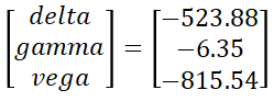
The goal is to find the weights of the three assets we are capable of trading to neutralize these values.
First, we will look to neutralize gamma and vega, then using the underlying asset, we will neutralize delta.
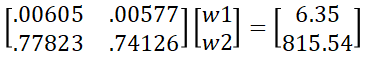
This means by inverting the matrix containing the greek values for the tradable options we can find the appropriate weights.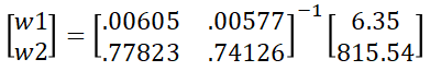
this is the code at ../deliverables/asset-allocation.py:
from src.utils import *from src.variables import *import numpy as np# Price option2 and option3 and find the greeksoption2 = EuropeanCall(asset_price=asset_price,asset_volatility=sigma,strike_price=K2,time_to_expiration=dt,risk_free_rate=rf)option3 = EuropeanCall(asset_price=asset_price,asset_volatility=sigma,strike_price=K3,time_to_expiration=dt,risk_free_rate=rf)# greek neutralization -- gamma and vegagreeks = np.array([[option2.gamma, option3.gamma], [option2.vega, option3.vega]])portfolio_greeks = [[option1.gamma * abs(nContract1)], [option1.vega * abs(nContract1)]]inv = np.linalg.inv(np.round(greeks, 2)) # We need to round otherwise we can end up with a non-invertible matrix# position on option 2 and 3 to be gamma and vega neutralw = np.dot(inv, portfolio_greeks)
Now that the exposure to gamma and vega is neutralized we need to neutralize our new exposure to delta.
To find our new exposure, we take the sum-product of all option positions in our portfolio with their respective deltas.
this is the code at ../deliverables/asset-allocation.py:
# Greeks including deltaportfolio_greeks = [[option1.delta * nContract1], [option1.gamma * nContract1], [option1.vega * nContract1]]greeks = np.array([[option2.delta, option3.delta], [option2.gamma, option3.gamma], [option2.vega, option3.vega]])w_stock = (np.round(np.dot(np.round(greeks, 2), w) + portfolio_greeks))[0]
the final positions are the following:
>>> Final asset allocation:option1: -1000option2: 8641option3: -8006underlying asset: -46
In this project, I’ve learned how to build Delta, Gamma and Vega neutral Portfolio to hedge the exposure against changes in volatility, movements in the underlying asset and the speed of movements in the underlying asset.
The code can be implemented directly into a live trading system in order to actively hedge the portfolio position day by day.
Hedging all Greek letters may require option positions greater than the original position.
Because of the limitations (instantaneous, local measures, model risk) of Greek letter hedging, this may rather increase than decrease risk.
The material discussed in this project it’s not financial advice.
This configuration has been tested against Python 3.8