Linear-and-Logistic-Regression

Linear-and-Logistic-Regression

This is my implementation of Linear Regression and Logistic Regression using python and numpy.

The goal of this project is to Implement Linear Regression and Logistic Regression #DataScience using NumPy Library.

Few popular hashtags -

#Linear Regression #Logistic Regression #Python

#Machine Learning #Data Analysis #Housing Dataset

Motivation

In this work, I used two LIBSVM datasets which are pre-processed data originally from UCI data repository.

1. Linear regression - Housing dataset (housing scale dataset). Predict housing values in suburbs of Boston. https://www.csie.ntu.edu.tw/~cjlin/libsvmtools/datasets/regression/housing_scale.
2. Logistic regression - Adult dataset (I only use a3a training dataset). Predict whether income exceeds $50K/yr based on census data. https: //www.csie.ntu.edu.tw/~cjlin/libsvmtools/datasets/binary/a3a

About the Project

Linear Regression:

1. Linear Regression is one of the most simple Machine learning algorithm that comes under Supervised Learning technique and used for solving regression problems.

2. It is used for predicting the continuous dependent variable with the help of independent variables.

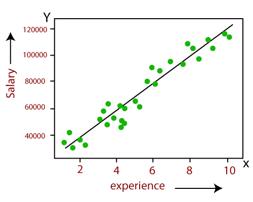
The goal of the Linear regression is to find the best fit line that can accurately predict the output for the continuous dependent variable

1. If single independent variable is used for prediction then it is called Simple Linear Regression and if there are more than two independent variables then such regression is called as Multiple Linear Regression.

2. By finding the best fit line, algorithm establish the relationship between dependent variable and independent variable. And the relationship should be of linear nature.

3. The output for Linear regression should only be the continuous values such as price, age, salary, etc. The relationship between the dependent variable and independent variable can be shown in below image

Logistic Regression:

1. Logistic regression is one of the most popular Machine learning algorithm that comes under Supervised Learning techniques.

2. It can be used for Classification as well as for Regression problems, but mainly used for Classification problems.
   Logistic regression is used to predict the categorical dependent variable with the help of independent variables.

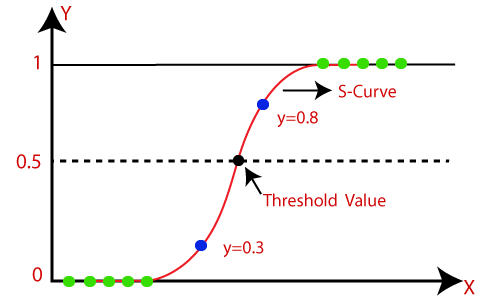
The output of Logistic Regression problem can be only between the 0 and 1.

1. Logistic regression can be used where the probabilities between two classes is required. Such as whether it will rain today or not, either 0 or 1, true or false etc.

2. Logistic regression is based on the concept of Maximum Likelihood estimation. According to this estimation, the observed data should be most probable.

3. In logistic regression, we pass the weighted sum of inputs through an activation function that can map values in between 0 and 1. Such activation function is known as sigmoid function and the curve obtained is called as sigmoid curve or S-curve. Consider the below image:

Steps involved in this project

Problem 1

Linear regression. I randomly split the dataset into two groups: training (around 80%) and testing (around 20%). Then I learn the linear regression model on the training data, using the analytic solution.

def lin1(x, y):
    n = int(x.shape[0])
    k = int(0.8*n)
    eresult = []
    costresult = []
    for j in range(10):
        a = range(n)
        np.random.shuffle(a)
        b = a[:k]
        c = a[k:]
        x_trn = x[b,:]
        x_tst = x[c,:]
        y_trn = y[b]
        y_tst = y[c]
        betta = analytic_sol(x_trn, y_trn)
        eresult.append(testError(x_tst, y_tst, betta))
        costresult.append(cost(x_tst, y_tst, betta))
    return eresult, costresult

After I compute the prediction error on the test data. I repeat this process 10 times and report all individual prediction errors of 10 trials and the average of them.

22.319096974362846
In this part of homework we can see that analytical solution is fast and effective method to solve this kind of problems. Problem 1 was relatively easy. I spent most of the time on setting up python and getting used to new libraries.

Problem 2

Linear regression. I do the same work as in the problem #1 but now using a gradient descent. (10 randomly generated datasets in #1 should be maintained;

def gradientDescent(alpha, x, y, max_iter=10000):
    m = x.shape[0] # number of samples
    n = x.shape[1] # number of features
    x1 = x.transpose()
    b = np.zeros(n, dtype=np.float64)
    for _ in xrange(max_iter):
        b_temp = np.zeros(n, dtype=np.float64)
        temp = y - np.dot(b, x1)
        for i in range(n):
            b_temp[i] = np.sum(temp * x1[i])
        b_temp *= alpha/m
        b = b + b_temp
    return b

we will use the datasets generated in #1.) Here I am not using (exact or backtracking) line searches. I try several selections for the fixed step size.

Here error is 3.2280665573708696. It is close to analytic solution it is 3.3454514565852436. The difference can be explained by randomness of splits (since we computed there values in different functions). So we can conclude that gradiend descent performs as well as analytical solution in terms of error.
In [31]:
error_gradient 
Out[31]:
3.2280665573708696

Problem 3

Logistic regression. As in the problem #1, I randomly split the adult dataset into two groups (80% for training and 20% testing). Then I learn logistic regression on the training data.

def logGradientDescent(alpha, x, y, max_iter=100):
    m = x.shape[0] # number of samples
    n = x.shape[1] # number of features
    x1 = x.transpose()
    b = np.zeros(n)
    for _ in xrange(max_iter):
        b_temp = np.zeros(n, dtype=np.float64)
        temp = y - hypo(b, x1)
        for i in range(n):
            b_temp[i] = np.sum(temp * x1[i])
        b_temp *= alpha/m
        b = b + b_temp
    return b

This is similar gradient descent function with backtracking linear search. I used minus gradient of objective function as a direction. -1 is because objective function is negative of loglikelihood. I use standard algorith for backtracking linear search found in Wikipedia. No stopping condition except iteration number. Here I compare the performances of gradient descent methods i) with fixed-sized step sizes and ii) with the backtracking line search. I tried to find the best step size for i) and the best hyperparameters α and β for ii) (in terms of the final objective function values).

In [38]:
np.sum(error_fixed)/10
Out[38]:
0.17688692615795415
In [39]:
error_back
Out[39]:
[0.18053375196232338,
 0.16897196261682243,
 0.17457943925233646,
 0.17943925233644858,
 0.18654205607476634,
 0.18168224299065422,
 0.18093457943925234,
 0.17196261682242991,
 0.18242990654205607,
 0.17981308411214952]
In [40]:
np.sum(error_back)/10
Out[40]:
0.17868888921492393

Here we can see that erro of BLS is greater than that of fixed step. I already explained this in graph.

It was difficult homework because we haven’t covered any implementations of ML algorithms before. However it was very interesting to implement them myself. It took a lot of time to start homework because of setting up and getting used to environment and libraries. This homework helped me understand concepts we covered in class bette

Libraries Used

Installation

• Install pandas using pip command: import pandas as pd
• Install numpy using pip command: import numpy as np
• Install matplotlib using pip command: import matplotlib
• Install matplotlib.pyplot using pip command: import matplotlib.pyplot as plt
• Install load_svmlight_file using pip command: from sklearn.datasets import load_svmlight_file

How to run?

Project Reports

• Download for the report.

Useful Links

1. Linear Regression Datasethttps://www.csie.ntu.edu.tw/~cjlin/libsvmtools/datasets/regression/housing_scale.
2. Logistic regression Dataset - https: //www.csie.ntu.edu.tw/~cjlin/libsvmtools/datasets/binary/a3a

Report - A Detailed Report on the Analysis

Contributing

• Clone this repository:

git clone https://github.com/iamsivab/Linear-and-Logistic-Regression.git

• Check out any issue from here.

• Make changes and send Pull Request.

Need help?

Feel free to contact me @ balasiva001@gmail.com

License

MIT © Sivasubramanian